Max De Marzi

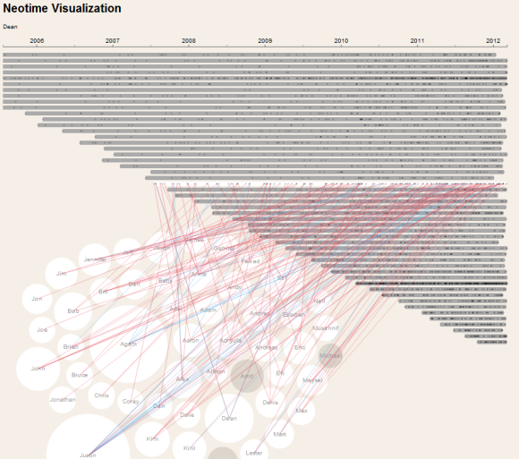
Some relationships change over time. Think about your friends from high school, college, work, the city you used to live in, the ones that liked you ex- better, etc. When exploring a social network it is important that we understand not only the strength of the relationship now, but over time. We can use communication between people as a measure.

I ran into a visualization that explored how multiple parties where connected by communications in multiple projects. We’re going to reuse it to explore how multiple people interact with each other. So let’s make a network of 50 friends and connect them to each other multiple times. Think of it as people writing on your facebook wall.

We will use the names of the first 50 members of the Graph DataBase- Chicago Meet-Up group for our names, but we’ll need a way to generate random times and offset them to simulate when people joined the social network.

def generate_time(from = Time.local(2004, 1, 1), to = Time.now)
  Time.at(from + rand * (to.to_f - from.to_f)).strftime('%Y-%m-%d')
end

def time_offset(n)
    Time.local(2004, 1, 1) + ((60*60*24*58) * n)
end

Let’s give our network a little something special. In your group of friends, most are quiet, some mingle, and some are social butterflies. We’ll create a random function with a power law distribution to model our connections and add a few outliers.

def powerlaw(min=1,max=500,n=20,o=0.05)
    max += 1
    pl = ((max**(n+1) - min**(n+1))*rand() + min**(n+1))**(1.0/(n+1))
    rand > o ? (max-1-pl.to_i)+min : rand(max).to_i
end

The code to create a relationship is pretty simple, we’ll use the Batch commands again and reference the nodes we create.

def create_rel(from,to,start_date,end_date)
  [:create_relationship, "wrote", "{#{from}}", "{#{to}}", {:date => generate_time(start_date,end_date)}]
end

Let’s put it together to create our graph. In order for our data to make sense, we are limiting the messaging between people to when they were both using the social network. You’ll see this in the maximum of the two nodes being passed into our time_offset method.

def create_graph
  neo = Neography::Rest.new
  graph_exists = neo.get_node_properties(1)
  return if graph_exists && graph_exists['name']
  commands = []
  names = %w[Aaron Achyuta Adam Adel Agam Alex Allison Amit Andreas Andrey 
             Andy Anne Barry Ben Bill Bob Brian Bruce Chris Corey 
             Dan Dave Dean Denis Eli Eric Esteban Ezl Fawad Gabriel 
             James Jason Jeff Jennifer Jim Jon Joe John Jonathan Justin 
             Kim Kiril LeRoy Lester Mark Max Maykel Michael Musannif Neil]

  commands = names.map{ |n| [:create_node, {"name" => n}]}

  names.each_index do |from|
    commands << [:add_node_to_index, "nodes_index", "type", "user", "{#{from}}"]  
    powerlaw.times do
      to = rand(50)
      commands << create_rel(from,to,time_offset([from,to].max),Time.now) 
    end
  end
  batch_result = neo.batch *commands
end

Our visualization was built using D3.js and it makes a web request expecting to see a JSON object that looks like:

{"cases":[{"title":"Aaron",
           "initiated_at":"2005-01-14",
           "last_correspondance_at":"2012-02-14",
           "exchanges":[{"incoming":true,
                         "sender_or_recipent":"2",
                         "journal_date":"2007-04-09"},
                        {"incoming":true,
                         "sender_or_recipent":"2",
                         "journal_date":"2008-10-02"}]}],
"parties":[{"id":1,"name":"Aaron","value":60},
          {"id":2,"name":"Achyuta","value":144}]}

We spent some time getting our data into our graph, now let’s get it all back out. Instead of getting everything in one shot, we’ll split the work into 3 queries. The first one called get_parties will get the users of the social network using Cypher. Notice that to get the ID of a node we use the ID() function and not me.id. We are also using the count, min and max cypher aggregate functions to get the data we need.

def get_parties
  neo = Neography::Rest.new
  cypher_query =  " START me = node:nodes_index(type = 'user')"
  cypher_query << " MATCH (me)-[r?:wrote]-()"
  cypher_query << " RETURN ID(me), me.name, count(r), min(r.date), max(r.date)"
  cypher_query << " ORDER BY ID(me)"
  neo.execute_query(cypher_query)["data"]
end

We’ll write another query to get the incoming relationships for each node. We are using the collect function to get two arrays back, one for the ids of friends and one for the date of the relationships.

def get_incoming_matrix
  neo = Neography::Rest.new
  cypher_query =  " START me = node:nodes_index(type = 'user')"
  cypher_query << " MATCH (me)<-[r?:wrote]-(friends)"
  cypher_query << " RETURN ID(me), me.name, collect(ID(friends)), collect(r.date)"
  cypher_query << " ORDER BY ID(me)"
  neo.execute_query(cypher_query)["data"]
end

A second query gives us the outgoing relationships for each node. Notice we are ordering both queries by the ID function.

def get_outgoing_matrix
  neo = Neography::Rest.new
  cypher_query =  " START me = node:nodes_index(type = 'user')"
  cypher_query << " MATCH (me)-[r?:wrote]->(friends)"
  cypher_query << " RETURN ID(me), me.name, collect(ID(friends)), collect(r.date)"
  cypher_query << " ORDER BY ID(me)"
  neo.execute_query(cypher_query)["data"]
end

Now we put it all together by combining the parties and their exchanges into a JSON object.

get '/communication' do
  p = get_parties
  parties = p.map{|p| {"id" => p[0], "name" => p[1], "value" =>p[2]} }
  cases = p.map{|p| {"title" => p[1], "initiated_at" => p[3], "last_correspondance_at" =>p[4], "exchanges" => []} }
  
  gim = get_incoming_matrix
  gim.each_index do |im|
    sors = gim[im][2][1..(gim[im][2].size - 2)].split(", ")
    jds  = gim[im][3][1..(gim[im][3].size - 2)].split(", ")
    sors.size.times do |t|
      cases[im]["exchanges"] <<  {"incoming" => true, "sender_or_recipent" => sors[t], "journal_date" => jds[t]}  
    end
  end

  gom = get_outgoing_matrix
  gom.each_index do |om|
    sors = gom[om][2][1..(gom[om][2].size - 2)].split(", ")
    jds  = gom[om][3][1..(gom[om][3].size - 2)].split(", ")
    sors.size.times do |t|
      cases[om]["exchanges"] <<  {"incoming" => false, "sender_or_recipent" => sors[t], "journal_date" => jds[t]}  
    end
  end
  {:cases => cases, :parties => parties}.to_json
end

The string wrangling you see to populate sors and jds is necessary because Cypher returns an Array wrapped inside a string instead of a proper array. One day we’ll get proper JSON objects back and this ugly little hack won’t be necessary. Update: We won’t have to wait long, the fix has been committed. All of the code is available on github as usual and you can play with it live on heroku.

You can use this visualization in many situations. Use it to visualize github commits to multiple projects by your development team. Conversations on Twitter about a range of Topics. Wikipedia page edits, patient records, resource utilization, etc.

Credits:
This post is based on the work of Even Westvang and his SeePlan series. He will be open sourcing his work soon. Watch this space for a link.